A long while ago I had posted about how a "A Bunch of Weak Classifiers Working Together Can Outperform a Single Strong Classifier." Such a bunch of classifiers/regressors is called an ensemble. As mentioned in that post, bagging and boosting are two techniques that are used to create an ensemble of classifiers/regressors. In this post, I will explain how to build an ensemble of decision trees using gradient boosting. Before going into the details, however, let us first understand boosting, gradient boosting, and why the decision tree classifiers and regression trees are the most suitable candidates for creating an ensemble.
The individual units in an ensemble are known as weak learners. Such learners are brittle in nature, i.e. a small change in the training data can have a major impact on their performance. This brittle nature helps to ensure that the weak learners are not well-correlated with each other. The choice of the tree model for weak learners is popular because tree models exhibit decent brittleness and such models are easily trained without much computation effort.
Boosting is one technique to combine weak learners to obtain a single strong learner or model. Bagging is another such technique. In bagging, all weak learners learn in parallel and independent of other learners. Every learner in bagging looks at only a part of the training data or a subset of features or both. In boosting, the weak learners are build sequentially using the full training data and the results from the preceding weak learners. Thus, boosting builds an additive model and the output of the ensemble is taken as the weighted sum of the predictions of the weak learners.
In the original boosting algorithm AdaBoost, the successive weak learners try to improve the accuracy by giving more importance to those training examples that are misclassified by the prior weak learners. In gradient boosting, the results from the preceding weak learners are compared with the desired output to obtain a measure of the error which the next weak learner tries to minimize. Thus, the focus in gradient boost is on the residuals, i.e. the difference between the desired output and the actual output, rather than on those specific examples that were misclassified by the earlier learners. The term gradient is used because the error minimization is carried out by using the gradient of the error function. The sequence of successive trees are of identical depth from 1 (stump) to 4.
A Walk Through Example to Build a Gradient Boosted Regression Tree
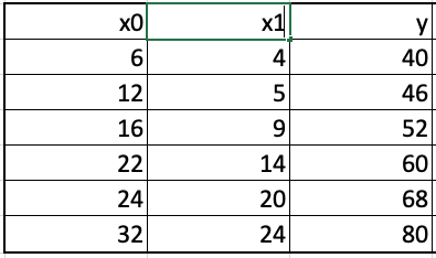
Let us work through an example to clearly understand how gradient boosted trees are build. We will take a regression example because building a gradient boosted regression tree is easier to understand than a gradient boosted classification tree. The example consists of two predictors, fertilizer input (x0) and insecticide input (x1), and the output variable is the crop yield (y). The goal is to build a gradient boosted regression tree to predict the crop yield given the input numbers for x0 and x1.
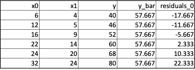
We will build a tree that minimizes the squared error (mse) between the actual output and the predicted output. We begin by building a base learner that yields the same prediction irrespective of the values of the predictor variables. This base prediction, let us denote it as y_hat_0, equals average of the output variable y, y_bar. Next, we calculate the residuals, the difference between the actual output y and the predicted output to obtain the residuals as shown below.
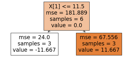
The next step is to adjust the predictions by relating the residuals with x0 and x1. We do this by fitting a regression tree to the residuals. We will use a tree of depth 1. To build the tree, we find the feature and the cut-off or the threshold value that best partitions the training data to minimize the mean squared error (mse). For the root node, such a combination consists of predictor x1 and the cut-off value of 11.5. The resulting tree is shown below. This tree was build using the DecisionTreeRegressor of the Sklearn library. Let's look at the meanings of different entries shown in the tree diagram. The mse value of 181.889 in the internal node of the tree is nothing but the error value if the residuals_0 column is approximated by the column average which is being shown by "value = 0." The number of examples associated with a node in the tree is given by "samples."
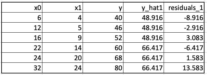
The above tree shows residual approximation by -11.667 for those training examples whose x1 value is less than or equal to 11.5 and the approximation by 11.667 when x1 is greater than 11.5. Assuming a learning rate of 0.75, we combine the above tree with the base tree (stump) to obtain updated predictions and the next set of residuals as shown below. To understand how the updated predictions were calculated, consider the predictor variables x0=6 and x1=4. The above tree tells us that for x1=4, the residual should be approximated by -11.667. The previous prediction for this particular x0,x1 combination is 57.667. Thus, the new prediction in this case becomes 57.667+0.75*(-11.667) which equals 48.916.
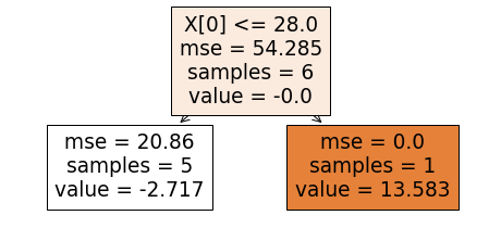
With the new set of residuals, we again build a tree to relate x0, x1 with residuals_1. This tree is shown below.
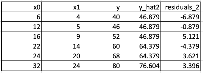
We update the predictions. For the first training example, the updating leads to the prediction 48.916+0.75*(-2.717) which equals 46.879. These updated predictions, y_hat2, and the new residuals, residuals_2 are shown below.
The tree building process continues in this fashion to generate either the specified number of weak learners or to the acceptable level of error.
Now that we know how gradient boosted trees are created, let us finish the above example using the GradientBoostingRegressor from the Sklearn library as shown below. The number of learners has been specified as 10 and the depth is set to 1.
import numpy as npfrom sklearn.ensemble import GradientBoostingRegressorfrom sklearn.metrics import mean_squared_error# Create data for illustrationX = np.array([[6,4],[12,5], [16,9],[22,14],[24,20],[32,24]])y = np.array([40, 46, 52, 60, 68,80])regressor = GradientBoostingRegressor( max_depth=1, n_estimators=10, learning_rate=0.75)gbt = regressor.fit(X, y)gbt.predict(X) |
array([40.18852649, 46.37977649, 49.56846063, 62.91676214, 67.36073713, 79.58573713]) |
How about Gradient Boosted Classification Trees?
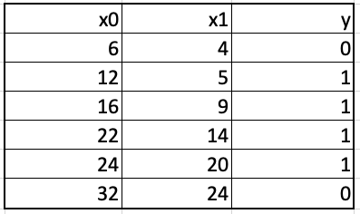
Let us convert the above regression example to a classification example by considering whether the crop yield was profitable or not based on fertilizer and insecticide costs. Thus, the output variable y now has two values, 0 (loss) and 1 (gain) as shown below.
Just like the procedure for building gradient boosted regression trees, we begin with a crude approximation for the output variable. The initial probability of class 1 over all the training examples, equal to 0.667, is taken as this approximation. The gradient boosted classifier is built using regression trees just like it is done while building gradient regression trees. The successive learners try to reduce the residuals, the difference between the y and the predicted probability.
Log Likelihood Loss Function and Log(odds)
The loss function minimized in the gradient boosted classification tree algorithm is the negative log likelihood. For a classification problem with two classes as we have, the negative log likelihood for the i-th training example is expressed by the following formula where p stands for the probability that the example is from class 1.
The loss is summed over all training examples to get the over all loss. The ratio p/(1-p) is called the odds or odds ratio, and often is expressed in terms of log(odds) by taking the natural log of the odds ratio. The probability p of an event and its log(odds) are related through the following equation:
Through some simple algebraic manipulation, we can also express the loss function as
Instead of calculating the gradient of the loss function with respect to p, it turns out that adjusting log(odds) offers a better way to minimize the loss function. Thus, taking the gradient of the loss function with respect to log(odd) results in the following expression:
The first term on the RHS of the equation is the negative of the desired output while the second term corresponds to the predicted probability (see the relationship between p and log(odds) above). The negative of the RHS in the above equation defines the residuals that we try to minimize by building successive trees via regression.
Back to Example
Coming back to our example, since the initial probability attached to every training example is 0.667 (ratio of class 1 labels and class 0 labels), the residuals are:
-0.667, 0.333, 0.333, 0.333, 0.333, -0.667
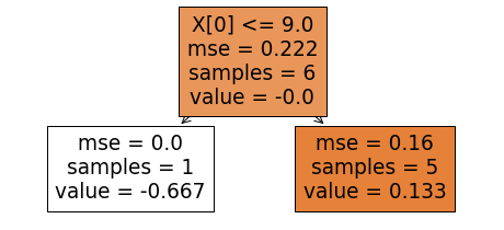
Let us try to fit a regression tree to the residuals at hand. Again, we will fit a tree of unit depth using the DecisionTreeRegressor from the Sklearn. The resulting tree shown below.
While in the case of the gradient regression trees, the "value" from the leaf nodes were directly used in the calculations of the updated residuals, we need to map "value" into log(odds) for calculating a new set of residuals in the present case. This mapping is done using the following relationship:
Let us try to understand the quantities in the RHS of the above expression. We will do so by referring to the right leaf node of the above tree. This leaf node has 5 samples that refer to the index "i" in the above expression. The item "value" in the leaf nodes is the residual for each example in the leaf node. There are five examples associated with the right leaf node; these are all but the first example of our data set. The previous probability is 0.667 for each of these examples. Thus, the mapped_log(odds) for these five examples are 5*0.133/(5*0.667*0.333), which equals 0.599. With 0.75 as the learning rate, the new log(odds) values for these five examples become 0.693(old log(odds)) + 0.75*(0.599) resulting in 1.142 for each of the five examples of the data set for which x0<9. Converting these log(odds) to probabilities, we see that 0.758 is the probability for the last five examples in the right leaf node to be from class 1. Carrying out similar calculations for the left leaf node, we end up with -1.559 as the updated log(odds) which translates to 0.174 as the probability that our first example in the data set is from class 1 or from the positive class.
Subtracting the updated probabilities from column y, we get a new set of residuals as shown below:
[-0.174, 0.242, 0.242, 0.242, 0.242, -0.758]
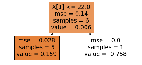
The regression tree built to fit these residuals is shown below.
We need to calculate the mapped_log(odds) again. The example associated with the right leaf in this case is the last example of the data set. The mapped log(odds) value for this example comes out as -4.132 following the formula for mapping shown above. The updated log(odds) value is then the 1.142(prior value) + 0.75* (-4.132). Converting the result into the probability, we get 0.123 as the probability that the last example in our data set comes from the positive class. Thus, it is classified as belonging to the negative (label 0) class. Let us now map the left leaf node value to log(odds) using the mapping formula.
= 5*0.159/((4*0.758*(1-0.758)+0.174*(1-0.174)))
= 0.906
This results in 0.906. Out of the five examples associated with the left leaf node, the four examples(all with y = 1) were together in the previous tree and had the updated log(odds) value 1.142 at that instance. The current log(odds) value for these four examples is then 1.142+0.75*0.906, equal to 1.821 which yields a probability value of 0.860. Thus, these four examples are correctly assigned the probability of 0.860 for the positive class. The remaining fifth example in the left node has a prior log(odds) value of -1.559. Thus, its updated log(odds) becomes -1.559+0.75*0.906, equal to -0.879. This gives 0.293 as the probability of this example from the positive class. Since the probability for the negative class is higher, this example is also correctly classified. At this stage, there is no need to add anymore learner because all examples have been correctly classified.
The above example was done to illustrate how the gradient boosted classifier builds its learners. Let us apply the GradientBoostingClassifier from the Sklearn library to check our step by step assembly of the learners explained above. We will print out the probability values to compare against our calculations.
from sklearn.ensemble import GradientBoostingClassifierclf = GradientBoostingClassifier( criterion='mse', max_depth=1, n_estimators=2, learning_rate=0.75)gbdt = clf.fit(X, y)list(gbdt.predict_proba(X)) |
[array([0.70657313, 0.29342687]),
 array([0.13928973, 0.86071027]),
 array([0.13928973, 0.86071027]),
 array([0.13928973, 0.86071027]),
 array([0.13928973, 0.86071027]),
 array([0.87645946, 0.12354054])]
You can see that these probabilities are identical to those calculated earlier. Thus, you now know how to build a gradient boosted classifier.
Before You Leave
Let us summarize the post before you leave. Boosting relies on an ensemble of trees to perform regression and classification. The gradient boosted trees for regression and classification give excellent performance. Using the Sklearn library without paying much attention to the number of learners and tree depth can lead to over-fitting; so care must be taken. One disadvantage common to all ensemble methods is that the simplicity of understanding model that one gets using a single tree is lost. A speedier and more accurate and scalable version of gradient boosted trees is the extreme gradient boosted trees (XGBoost). The performance of XGBoost algorithm is at par with deep learning models and this model is very popular.
Image
Insert an image to make a visual statement.
Settings
Leave empty if decorative.
Select the size of the source image.
